Posts Tagged ‘Excel’

h1

Word: Delete, add, or change author name

April 6, 2019

When you create a document in Microsoft Word, PowerPoint, or Excel, the user name you entered on File > Options > General tab is automatically added as the author name. In most cases, you want this. But what if you don’t? What if the author name is the name of the person who created the template you’re using? Or is the original creator of the document you’re modifying who left the organisation long ago? What if you want to remove that name altogether and add your own name (or some other name) as the author?

(NOTE: Be careful when changing the author name that you don’t break any copyright laws—these laws vary from country to country, but essentially, the author of a document is likely the copyright owner of that document, except perhaps in cases of ‘work for hire’ where the organisation owns the copyright. If in doubt, speak to a lawyer or the organisation’s Legal Department.)

This information applies from Word for Windows 2010 and later.

How to delete an author name in an Office document (Word, PowerPoint, or Excel)

  1. Open the document.
    NOTE: If you want to change the author name in a template, right-click on the template, and select Open to open the template. Do not double-click the template to open it as it will only open a document based on the template, not the template itself.
  2. Go to File > Info.
  3. Right click on the author’s name.
  4. Select Remove Person.

How to add an author name in an Office document (Word, PowerPoint, Excel)

  1. Open the document.
  2. Go to File > Info.
  3. Click Add an author.
  4. Type in the new name, or click the book icon to select it from your Contacts list.

How to change your name for future Office documents (Word, PowerPoint, Excel)

  1. Open a document.
  2. Go to the File > Options > General tab.
  3. Change your name in the User name field.
  4. Optional: Change your initials too.
  5. Click OK.
  6. Close the document.
  7. Check that the new name is applied to a new document—create a new blank document (not based on a template), then check the User name property under File > Options > General tab, and that it’s used as the author name when you go to File > Info.


h1

Excel: Convert hours and minutes to minutes

August 2, 2017

Converting hours and minutes (hh:mm) to minutes in an Excel spreadsheet is actually quite simple, once you know what to do. But I had to do quite a bit of trial and error and Googling to get it to work.

To convert hours and minutes to minutes, you have to multiply the hh:mm value by 1440 (which is 24 [number of hours in the day] multiplied by 60 [number of minutes in an hour]), AND make sure you set the formatting correctly for the both the hh:mm cells and the resulting minute cells. This is where I got caught — I didn’t have the correct formatting applied to the cells. Once I got that right, it all worked.

Here’s how…

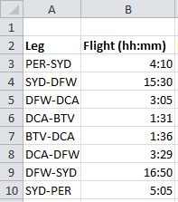
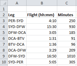
  1. Enter elapsed times in hours and minutes (using the format hh:mm) in Column B. (Yes, those non-stop flights to/from Sydney to Dallas Fort Worth are killers!)
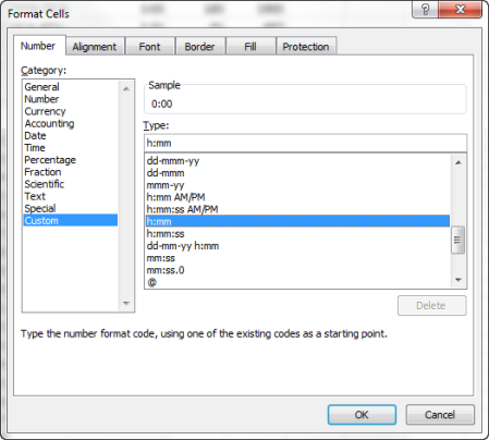
  2. Set the format for this column to Custom > h:mm. (To format the column, select the column header, right-click on it, select Format Cells, select Custom on the Number tab, then select h:mm from the list of types. Click OK.)
  3. Insert a new column (C) and called it Minutes.
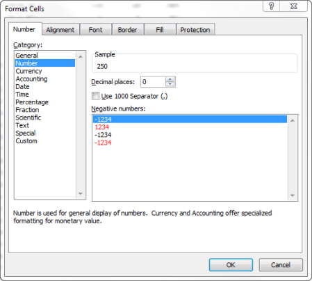
  4. Set the format for the cells in this new column to Number with no decimal places — this formatting is critical for the formula to work. (To format the column, select the column header, right-click on it, select Format Cells, select Number on the Number tab, then change the Decimal Places value to 0. Click OK.)
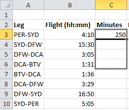
  5. Put the cursor in the first cell in the new column that pairs with a cell in the hh:mm column. In my example, that was C3, which pairs with B3.
  6. Type =B3*1440 in the formula bar, then press Enter to convert the hours and minutes into minutes.
  7. Click in the C3 cell and ‘grab’ the bottom right handle of the cell marker (it turns to a + sign when you’ve grabbed it correctly) and drag it down the other cells in column C. (See below for how to apply it to ALL cells in the column.)

  8. When you release the mouse, all those cells you dragged this formula over will be converted to minutes and seconds.

To apply this formula to the entire column:

  1. Copy (Ctrl+C) the result in the first cell with the formula (C3 in my example).
  2. Select the entire column (column C in my example) by selecting the column header.
  3. Paste (Ctrl+V).
  4. You’ll have to rename the column back to Minutes, but you’ll have that formula now applied to every row of your spreadsheet for that column.

These sites helped me figure out what to do:

See also:

[Links last checked August 2017]

h1

Excel table into Word — quick and easy method!

August 25, 2014

I’ve written before about some methods for getting the data in an Excel spreadsheet into Word (see the links below).

Recently, one of my colleagues had a BIG Excel spreadsheet table (all text) that had to be inserted into a Word document. In this instance, inserting a link to the spreadsheet was not an option, and saving it as multiple images and inserting those was problematic too (fuzzy, almost unreadable text mostly). So in despair my colleague asked me for some help.

In the process of testing many options I stumbled on a solution, but then I forgot which of the many combinations of things I tried was the one that worked ;-) So after a bit more testing I got it to work again.

Here’s how:

  1. Save the Excel spreadsheet as either a MHT or HTM file (doesn’t matter which – both work).
    excel_word01
  2. Open this saved file in Internet Explorer. Right-click on the saved file, then select Open with > Internet Explorer. NOTE: This method DOES NOT work if you open it in another browser, such as Firefox or Chrome — you must open it in Internet Explorer.
  3. In Internet Explorer, go to File > Edit in Word (or similar), which opens the spreadsheet in Word as a table. (If you can’t see File, press the Alt key to show the menu.)
  4. You may have a little bit of fiddling to do (e.g. remove blank columns, resize columns, change font size), but it shouldn’t be much.
  5. Select the reformatted table, copy it, then paste it into your main Word document (or save it as a new document if you aren’t inserting it into another document).

See also:

[Links last checked August 2014]

h1

Word: Getting an Excel table into Word

July 10, 2013

Typically, you have two choices when you want to insert an unlinked Excel table into a Word document:

The choice you make will depend on what you need to do – or not do – with the data once it’s in Word. If you don’t need to modify it, then insert it as an image; if you do need to modify it, then insert it as a Word table.

Related articles:

For inserting a linked table and other options see: http://office-watch.com/2016/putting-excel-into-word/

[Links last checked July 2103; based on a Writing Tip I wrote for my work colleagues]

h1

Excel: Convert seconds to minutes

April 27, 2012

You’d think that converting seconds to minutes in an Excel spreadsheet would be simple, but it’s not. You can’t just divide by 60 — the result of that will be minutes and decimal fractions of a minute, not minutes and seconds. For example, if you divide 78 seconds by 60, you get 1.3, but 1.3 is NOT the same as 1:18 (1 minute and 18 seconds). Likewise, 247 seconds divided by 60 is 4.11, whereas 247 seconds is actually 4 minutes and 7 seconds. If you only have a couple to do, no big deal — just figure it out in your head. But if you have hundreds or thousands of these conversions, you need a formula for doing that.

To convert seconds to minutes, you have to divide the seconds by the total number of seconds in a day, then tell Excel to display the result in mm:ss format. Simple, huh? ;-)

Here’s what I did…

  1. Column G in the screen shot below has a long list of seconds. Because I need to reference column G and put the results into a new column, I inserted a new column (H) and called it mm:ss.
  2. However, inserting a new column isn’t enough — I have to format the cells in that column so that they display the result in minutes and seconds. To format the column, select the column header, right-click on it, select Format Cells, select Custom on the Number tab, then select mm:ss from the list of types. Click OK.
  3. Go to the first cell in the new column that pairs with a cell in the seconds column. In my example, that was H4.
  4. In the formula bar, type =G4/86400 then press Enter. The seconds convert into minutes and seconds! (But where does that 86400 come from? That’s the number of seconds in a day — 60 x 60 x 24 = 86400. And the G4 was the reference cell for my H4 cell.)
  5. Now, click in the H4 cell and ‘grab’ the bottom right handle of the cell marker and drag it down the other cells in column H. (See below for how to apply it to ALL cells in the column.)

  6. When you release the mouse, all those cells you dragged this formula over will be converted to minutes and seconds.

To apply this formula to the entire column:

  1. Copy (Ctrl+C) the result in the first cell with the formula (H4 in my example).
  2. Select the entire column (column H in my example) by selecting the column header.
  3. Paste (Ctrl+V).
  4. You’ll have to rename the column back to mm:ss, but you’ll have that formula now applied to every row of your spreadsheet.

These sites helped me figure out what to do:

[Links last checked April 2012]

h1

Excel doesn’t allow you to view or specify keyboard shortcuts

February 1, 2012

One of the things I like about Word is that you can specify your own keyboard shortcuts for your macros and for functions that don’t already have a key combination. Or you can modify those that are already assigned in Word (though I wouldn’t advise it, because if you have to reinstall Word or you use someone else’s machine your keyboard shortcuts won’t work the same as the ones you’ve set up for your installation of Word).

Assigning keyboard shortcuts has been a feature in Word for years, and I just assumed that the other Office products would have similar functionality. Not so. I was alerted to this lack because of a comment on one of my blog postsCtrl+Shift+C activates the Format Painter in Word, but doesn’t do so in Excel, even though Excel also has the Format Painter function.

Microsoft Excel 2010 (and likely earlier versions), does NOT have any option available to view existing key combinations or to create your own. And on further investigation nor does PowerPoint 2010, Visio 2010, or Outlook 2010 (I didn’t check all the Office programs).

For example, here’s the Word 2010 screen with the option to assign a keyboard shortcut (found under File > Options > Customize Ribbon):

Word 2010 allows you to assign a keyboard shortcut

Word 2010 allows you to assign a keyboard shortcut

And here’s the same screen in Excel 2010 — nothing!:

Excel 2010 doesn't let you to assign a keyboard shortcut

Excel 2010 doesn't let you to assign a keyboard shortcut

I think this is a really big oversight by the Microsoft Office team. Those who use these products all day, every day, can be incredibly efficient using keystrokes instead of the mouse. I can’t believe that Microsoft has denied users the ability to add their own to existing functions.

Note: I understand that you can still assign a keyboard shortcut to a macro you create in Excel etc.

See also:

[Links last checked January 2012]

h1

Excel was around before electricity!

September 8, 2011

How else can you explain this from the Excel 2007 recovery window? 1601? Really??

h1

Excel: Force a line break in a text cell

September 5, 2011

Need to force a line break in an Excel cell?

Just press Alt+Enter where you want the line break to go.

This also works for Excel data used in Word mail merge fields — you can force the text in the mail merge to go onto another line by adding the line break in the Excel cell containing the data. Very handy for a multi line address when you only have, say, two or three cells for the address fields but need four or five lines for some addresses.

h1

Excel: Save a worksheet as an image file

June 29, 2011

You can save an Excel worksheet to several formats, but, surprisingly, you cannot save it — or a selection from it — as an image. I would have thought this simple function would have been an option in Excel 2007 or 2010, but it’s not.

Saving to PDF (and then to an image format) is an option if the worksheet is not particularly wide, but as soon as the worksheet stretches over more than one page, PDF is not suitable unless you want to cobble together several PDF files to make one image.

After trying several methods and searching the internet, I figured out the best way to do it; this method works in Excel 2003, 2007, and 2010:

  1. Select the worksheet cells containing the data, chart, etc. you want to save as an image (turn off grid lines if you don’t want them too).
  2. Copy the selection to the clipboard (Ctrl+C).
  3. Open a graphics editor. My personal preference is SnagIt, but Microsoft Paint works just as well.
  4. Paste the selection into your graphics editor (Ctrl+V).
  5. Save the pasted image as a GIF (suitable for simple line drawings), JPG (suitable for photos only), or PNG (suitable for almost anything).

From my internet searching, it sounds like this is something many people want to do, so it would be good if Microsoft could offer a ‘save as image’ option from Excel.

Aside: Some wit on the internet had this to say about how to save an Excel worksheet as an image:

Take a photograph using your phone, send it to your home email,  then sketch an artist’s impression of said Excel sheet based on the photo content, scan that into your hard drive, send back to work and save it.

Another had this method:

  1. Stick a sheet of tracing paper to your monitor.
  2. Then make a brass rubbing of the Excel table.
  3. Remove the tracing paper and pour plaster of paris over the top.
  4. Cover in spray mount and glitter.
  5. Shake off the excess and voila!

[Link last checked June 2011]

h1

Excel: Reference lists in another worksheet

June 9, 2011

Scenario

I was asked to set up a mail merge letter for my client. I knew I could create a ‘database’ in Excel and refer to that for the mail merge fields in the Word document. However, some of the fields would have data in them that would be used in every letter, and this data was ideal for a drop-down selection list.

Such selection lists simplify the process for the person entering the data in the Excel spreadsheet, save them time, and make the data entry more accurate as they can’t make spelling errors or typos.

For example, one of the mail merge fields I created was for the type of document that was referred to in the letter; the only acceptable document types were:

  • Appendices
  • document
  • Plan
  • Program
  • Report
  • Supplement

I knew I could create the data lists for the drop-downs in Excel (thanks to a great session on just this by Michael Hughes at the 2009 WritersUA Conference), but I wanted them on their own worksheet, and I wasn’t sure how to reference them from the data entry sheet (I’m an Excel novice!).

Solution

In this tutorial, I’ll show you how to set up a list in Excel 2007 and how to reference it from cells on the main data entry worksheet.

Bottom line: Reference cells in another worksheet by adding the worksheet name plus an exclamation mark between the = sign and the cell range (e.g. =Lists!$A$2:$A$7 for a range of cells on the Lists worksheet).

Step 1: Name the worksheets

  1. Open a new Excel document.
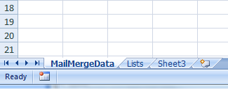
  2. Change the name of Sheet1 to MailMergeData — this will be the data entry sheet.
  3. Change the name of Sheet2 to Lists — this sheet will contain the list items for the various fields.
  4. Save the document. For this example, call it MailMergeData.xlsx.
Change the names of the worksheets

Step 2: Name the data columns

  1. Go to the MailMergeData sheet.
  2. In Row 1, enter the names of the data fields that you’ll use in your mail merge letter — one in each cell. Don’t use spaces, symbols or punctuation in the names, and don’t duplicate any names — each has to be unique. Try to make the names meaningful and recognizable; these names will be listed in the mail merge field selection list, so you need to be able to figure out what they are. (In the screen shot below, I’ve used RecFirstName and RecLastName for the recipient’s first and last names, RecOrganization for the recipient’s organization, DocType for the type of document.)
  3. For ease of reading, format Row 1 so that the field names are obvious (e.g. increase the font size, add a background color, make the font bold, etc.).
  4. Save the document.

Step 3: Set up the list items for the selection lists

  1. Go to the Lists worksheet.
  2. In Row 1, Column A, type the name of the data field for that particular list (this name is only for you/someone else to identify at a later date — it isn’t used in the mail merge nor is it critical to the drop-down lists you create; I tend to use the same name as that in the MailMergeData sheet, but this isn’t essential.)
    Item list
  3. Move to the next column in Row 1 and type the name of the next data field that will have a drop-down list.
  4. Repeat step 3 for as many lists as you need to create; remember, not every data field in your mail merge dataset will have a selection list.
  5. For ease of reading, format Row 1 so that the field names are obvious (e.g. increase the font size, add a background color, make the font bold, etc.).
  6. Underneath Row 1, Column A, type each list item, one per cell. Try to keep them in alphanumeric order as neither Excel nor Word sorts them automatically.
  7. Add the list items for the other data fields.
  8. Save the document.

Step 4: Find and select the list item range

Next you’ll select each list item range to find out their row and column values.

  1. Go to the Lists worksheet.
  2. On the Data tab, click the Data Validation button, then select Data Validation. This opens the Data Validation dialog box.
  3. In the Allow field on the Settings tab, select List.
    Data Validation dialog box
  4. Click the icon to the right of the Source field to open a small Data Validation window.
    Data Validation panel
  5. Select all the items in one of your lists by clicking and dragging your cursor over those cells.
  6. As you do this, the selection is shown in the Data Validation field as something like =$A$2:$A$7, which indicates everything in column A, rows 2 to 7 inclusive, as shown in the example below.
    Selected items as displayed in the Data Validation panel
  7. Press Enter to show the full Data Validation dialog box. The cell range is displayed in the Source field.
  8. Select everything in the Source field and copy your selection to the clipboard.
  9. Click Cancel as you don’t need this dialog box again for this list.

Step 5: Add the list item range to the mail merge field

In this step, we’ll select the field in the MailMergeData worksheet and use data validation to link to the other worksheet’s item list.

  1. Go to the MailMergeData worksheet.
  2. Select the first empty cell in the column where you want the drop-down list to go. In the example below, I selected the first cell under the DocType heading.
  3. On the Data tab, click the Data Validation button, then select Data Validation. This opens the Data Validation dialog box.
  4. In the Allow field on the Settings tab, select List.
  5. In the Source field, paste in the range you copied to the clipboard a few seconds ago.
  6. Put your cursor IMMEDIATELY after the = sign, and type Lists! You should end up with something like: =Lists!$A$2:$A$7 (Lists is the name of the worksheet you are referencing and the ! tells Excel to look for that cell range on the Lists worksheet, not the current one. Make sure you type the worksheet name correctly, otherwise it won’t work — List is not the same name as Lists.)
    Data Validation dialog box with reference to other worksheet
  7. Click OK to save your changes and close the Data Validation dialog box.
  8. As soon as you click OK, you should see a drop-down arrow next to the cell you’re in.
  9. Click the arrow to test that the list displays as you expect it to.
    Drop-down list referenced from other worksheet
  10. If it works as you expect, apply this range to other cells in this column by dragging the little square icon at the bottom right of the cell down the column to cover as many rows as you want. For example, if your mail merge dataset typically has 20 individuals, then drag it down 20 rows.
    Drag the settings to other cells in this column
  11. Save your changes.

Quick way to link to the same list range but for different columns

If you have several lists set up on the Lists worksheet, then instead of going through many of the steps above, you can just do the steps once, then, once you have your initial range (e.g. =Lists!$A$2:$A$7), you can copy that into other Data Validation dialog boxes and change the column letter and row numbers to reflect the other list. For example, let’s say you have another set of items for a drop-down list that are in column E, rows 2 to 12 — change the ‘A’ in =Lists!$A$2:$A$7  to ‘E’ and the ‘7’ to ’12’, giving you =Lists!$E$2:$E$12. Leave everything else as it is.

Alternative method

Based on the post above, Peter Sanders made this short video on using Range Names instead: http://www.screencast.com/t/jKKSD7zeDzac Being an Excel novice, I knew there would be a more elegant solution than mine, and Peter has provided it. Thanks for your contribution, Peter!

See also:

[Links last checked June 2011; thanks to @michaelhughesua for his conference session related to this, and to Peter Sanders for the video]